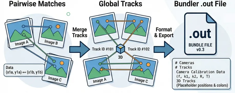
From Tie-Points to Global Tracks: Building Your Own Bundler File

If you work with Structure from Motion (SfM) or photogrammetry, you’ve probably run into the Bundler format (.out). It’s the standard way to store 3D feature tracks alongside camera calibrations, and it’s one of the few ways that I know how to to import your own tie-points into Agisoft Metashape.

And that is what I needed for my project! I had my own tie-point matching pipeline producing pairwise matches, and I wanted to get those into Metashape for further processing. The only way in? A Bundler file. So I decided to build one from scratch. In an upcoming post I’ll show the Metashape side — how to actually load the bundler file correclty and work with it. Today is about everything that happens before that: going from raw pairwise matches to a clean, valid Bundler file.

The pipeline

Starting point

A normal feature matching pipelines give you matches between pairs of images. For each pair you get a set of corresponding pixel coordinates, confidence scores, and (optionally) feature descriptors. Something like:

Image A ↔ Image B:  [(x1a, y1a) → (x1b, y1b), conf=0.95],
                    [(x2a, y2a) → (x2b, y2b), conf=0.87], ...

Image A ↔ Image C:  [(x1a, y1a) → (x3c, y3c), conf=0.91], ...

The problem is that these pairs don’t know about each other. Point (x1a, y1a) in Image A might appear in matches with Image B and Image C, but nothing connects those two matches yet. To build a 3D reconstruction, we need global tracks — a single track ID that says “this is the same physical point, seen in images A, B, and C.”

Step 1: Flatten everything into arrays

The first thing we do is unpack all pairwise dictionaries into flat, pre-allocated NumPy arrays. Every observation (a point in a specific image) gets an initial track_idx — at this stage, each track connects exactly two points.

# Pre-allocate arrays for all observations
total_obs = sum(tps.shape[0] * 2 for tps in tp_dict.values())

x_arr       = np.empty(total_obs, dtype=np.float32)
y_arr       = np.empty(total_obs, dtype=np.float32)
img_idx_arr = np.empty(total_obs, dtype=np.int32)
track_arr   = np.empty(total_obs, dtype=np.int64)

track_counter = 0
for (img1_id, img2_id), tps in tp_dict.items():
    n = tps.shape[0]
    pts1, pts2 = tps[:, :2], tps[:, 2:]

    # Both points in a pair share the same track_idx
    track_arr[idx:idx+n]     = np.arange(track_counter, track_counter + n)
    track_arr[idx+n:idx+2*n] = np.arange(track_counter, track_counter + n)

    track_counter += n

Pre-allocating matters here. With tens of thousands of matches across hundreds of image pairs, you don’t want to be appending to Python lists.

Step 2: Spatially-aware merging with descriptors

Now comes the core challenge: figuring out which of these two-point tracks are actually the same physical feature and should be merged. For each image, we take all observed points and build a KD-Tree to find candidates that are spatially close (within a configurable pixel tolerance):

from scipy.spatial import cKDTree

coords_normalized = coords / float(max(width, height))
tolerance_normalized = px_tolerance / float(max(width, height))

tree = cKDTree(coords_normalized)
pairs = tree.query_pairs(r=tolerance_normalized, output_type="ndarray")

But proximity alone isn’t enough. Two distinct features — say the corner of a window and the corner of a door frame — can land within a few pixels of each other in a given image. If we have feature descriptors available, we filter candidates by cosine similarity:

def _cosine_similarity(vec1, vec2):
    dot = np.dot(vec1, vec2)
    norm1, norm2 = np.linalg.norm(vec1), np.linalg.norm(vec2)
    if norm1 < 1e-8 or norm2 < 1e-8:
        return 0.0
    return dot / (norm1 * norm2)

# Only keep pairs where descriptors are similar enough
valid_pairs = [
    (i, j) for i, j in spatial_pairs
    if _cosine_similarity(descriptors[i], descriptors[j]) >= 0.85
]

The pipeline also works without descriptors (proximity-only merging), but you’ll get cleaner tracks with them.

Step 3: Cross-image consistency checks

This is where most homegrown pipelines fall apart, and where I spent the most debugging time. Imagine Track A and Track B look like they should merge in Image 1 — they’re close together and their descriptors match. But both tracks also appear in Image 2, and there they’re 200 pixels apart. Merging them would create a physically impossible track. Before any merge is finalized, we check every other image where both tracks have observations:

# From _merge_points_checked() — the cross-image safety net
obs_i = track_obs.get(track_idx_i, {})  # {image_idx: (x, y)}
obs_j = track_obs.get(track_idx_j, {})
shared_images = set(obs_i.keys()) & set(obs_j.keys())
shared_images.discard(current_image_idx)

if shared_images:
    consistent = True
    for img in shared_images:
        xi, yi = obs_i[img]
        xj, yj = obs_j[img]
        dist = ((xi - xj)**2 + (yi - yj)**2) ** 0.5
        if dist > px_tolerance:
            consistent = False
            break
    if not consistent:
        continue  # reject this merge

This check is cheap but catches a surprising number of bad merges. In my datasets, typically 5–15% of spatially valid candidates get rejected here.

Step 4: Resolving merge chains with Union-Find

Merging is transitive. If track 1 merges with track 2, and track 2 merges with track 3, then all three belong together. Naively storing parent[old] = new breaks when the same track gets merged from multiple images in the same iteration — the second write overwrites the first. The solution is a proper Union-Find with path compression:

def _resolve_mapping_chains(mappings):
    parent = {}

    def find(x):
        if x not in parent:
            parent[x] = x
        path = []
        r = x
        while parent[r] != r:
            path.append(r)
            r = parent[r]
        for node in path:
            parent[node] = r  # path compression
        return r

    def union(a, b):
        ra, rb = find(a), find(b)
        if ra != rb:
            # Smaller ID becomes root (deterministic)
            if ra < rb:
                parent[rb] = ra
            else:
                parent[ra] = rb

    for old, new in mappings:
        union(int(old), int(new))

    # Build final mapping
    return {
        node: find(node)
        for node in {int(x) for pair in mappings for x in pair}
        if node != find(node)
    }

After resolving chains, we apply the mapping to the DataFrame, drop duplicate observations (keeping the one with highest confidence), and discard orphan tracks that appear in fewer than two images. The whole merge process runs iteratively — each pass may unlock new merge candidates that weren’t adjacent before. It converges when no new merges are found.

Step 5: Writing the Bundler file

With clean global tracks in hand, the export is mostly formatting. But there are a few things to get right:

Coordinate conversion.
Bundler uses a centered coordinate system where (0, 0) is the image center, with y pointing up. Most feature detectors use top-left origin with y pointing down:

bundler_x = x - image_width / 2.0
bundler_y = image_height / 2.0 - y

The file structure.
A bundler.out file has a strict layout:

# Bundle file v0.3
<num_cameras> <num_tracks>

# For each camera:
<focal_length> <k1> <k2>
<r00> <r01> <r02>
<r10> <r11> <r12>
<r20> <r21> <r22>
<t0> <t1> <t2>

# For each track:
<x> <y> <z>          (3D position — we use 0,0,0 as placeholder)
<r> <g> <b>          (average color from source pixels)
<num_observations> <img_idx> <feature_idx> <bx> <by> ...

The companion
This is easy to overlook but critical. It maps camera indices to image filenames — without it, Metashape guesses the association by load order, which breaks if your images weren’t added in the same sequence. So you need to create a list.txt.

with open(list_path, "w") as lf:
    for p in img_paths:
        lf.write(p + "\n")

The calibration data
The Bundler format normally requires camera parameters (focal length, radial distortion, rotation, and translation) for every image. If you are exporting from a system that has already performed some reconstruction (like COLMAP), you can pipe those values directly into the file. However, if you are just trying to get your manual matches into Metashape to start a reconstruction, these values act as your initial guess.

The final result

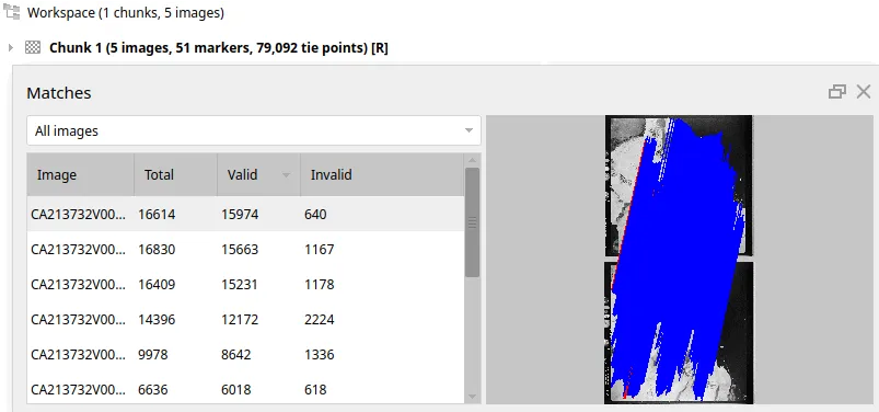
And just like that, we’ve turned a mess of pairwise guesses into a globally consistent map. It’s alive! Loading the result into Metashape shows just how dense our custom pipeline can get:

What’s next

In the next post, I’ll walk through the Metashape side: how to import a Bundler file, what settings matter, and how to go from imported tie-points to a dense point cloud. If you’re building something similar or have questions about the pipeline, feel free to reach out.