Matching Massive Images: A Tiled Pipeline for LightGlue and RoMa

In my last post, we covered turning pairwise matches into a Bundler .out file. But that assumes you already have high-quality matches—which isn’t always a given.

When working with large-scale historical imagery (in my case, archival aerial imagery of Antarctica), standard tools like SIFT often fail against textureless ice and film degradation. The modern solution is to use deep learning models like SuperPoint and LightGlue. However, feeding massive, high-res scans directly into your GPU is often not feasible—you have to bridge the gap between image size and match quality.

This post walks through two different methods I built for getting reliable matches out of large images. It’s code-heavy, with extensive examples. A full notebook will be soon available.

The Basics

Before diving into the code, let’s establish some terminology. Points
In photogrammetry, “points” refer to specific image locations of interest for matching. There are two main types:

• Keypoints (KPs): Distinct 2D pixel coordinates identified in a single image—like the sharp corner of a building.
• Tie Points (TPs): Matched keypoint pairs between two different images, also called “matches” or “correspondences.” These represent the same physical location in the real world seen from two different viewpoints, and they are ultimately what photogrammetry needs.

Matchers
Matchers are algorithms or neural networks that take keypoints and their descriptors from two images and find correspondences between them. They analyze the descriptors to determine which keypoints from Image A likely correspond to which keypoints in Image B, based on similarity and geometric consistency.

• SIFT: The classic workhorse of computer vision. Unlike the modern tools on this list, SIFT is not a neural network—it relies on traditional gradient math to find edges and corners. While incredibly reliable and still the default in many commercial photogrammetry applications, it can struggle with extreme lighting changes, heavy shadows, or severe perspective shifts where deep-learning methods excel.

• SuperPoint & LightGlue: The modern gold standard for sparse matching. SuperPoint acts as the “scout”—a CNN that extracts highly distinct keypoints and their unique descriptors. LightGlue (the successor to SuperGlue) is the “cartographer,” matching those descriptors using a fast transformer architecture.

• RoMa: Where SuperPoint/LightGlue focus on specific, isolated points (sparse matching), RoMa analyzes the entire image patch to estimate pixel-to-pixel warps (dense matching). Because it considers the whole area holistically, it is highly robust against extreme viewpoint shifts, drastic lighting changes, and mostly textureless surfaces.

Homography & Geometric Filtering
Both approaches rely heavily on computing a homography—a mathematical mapping that describes how the flat surface of Image 1 relates to Image 2. We use this both to predict where tiles should overlap and as a final filter to remove false positive matches (outliers).

Throughout these pipelines, I use USAC_MAGSAC instead of classic RANSAC. MAGSAC++ is threshold-free and marginalizes over noise levels, making it significantly more robust against the noise inherent in high-res imagery.

# A standard robust homography calculation used throughout this pipeline
h_matrix, inlier_mask = cv2.findHomography(
    pts1, pts2,
    method=cv2.USAC_MAGSAC,
    ransacReprojThreshold=5.0,
    confidence=0.9999,
    maxIters=10000,
)

The Two Approaches

I ended up building not one but two different pipelines. Approach 1 is the more classic “extract & match” pipeline. Approach 2 grew from the need to handle more extreme geometric changes and achieve subpixel accuracy, combining two different matchers.

Both have distinct advantages depending on the scenario:

	Approach 1: Two Stages	Approach 2: One Stage
Speed	Faster	Slower (RoMa is computationally heavy)
Reusability	High (keypoints can be reused across pairs)	Low (keypoints computed on-the-fly)
Subpixel Accuracy	No*	Yes (RoMa achieves subpixel accuracy)
Complexity	Higher (separate extraction and matching phases)	Lower (directly finds tie points)
Robustness	Moderate (depends on LightGlue’s performance)	High (RoMa handles extreme cases well)
Match Volume	Moderate	High

*See Tips & Tricks for a post-processing workaround.

---

Approach 1: The Two-Stage “Extract & Match” Pipeline

This is the classic approach: find all interesting points in Image A, find all interesting points in Image B, then compare the two sets. The key advantage is reusability—if you match the same image multiple times (e.g. Image A → B, then Image A → C), you only extract keypoints from Image A once and reuse those descriptors for every subsequent pair.

Finding Keypoints

Phase 1: Preparation & Tiling
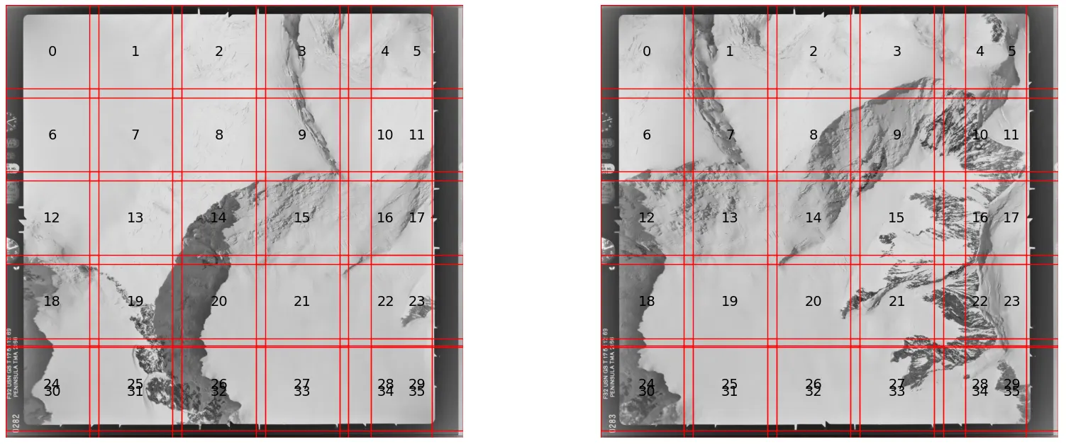
The image is converted to 2D grayscale and checked against the minimum size requirements for the neural network. To handle large images safely, it is divided into a grid of overlapping square tiles. Because we don’t yet know which region of the image will overlap with the second image, we tile the entire thing. Figure 1 shows an example. Tiles are designed to overlap by around 20% to ensure keypoints near tile edges are never missed. Where tiles don’t fit perfectly, those at the right and bottom edges extend further to ensure full coverage.

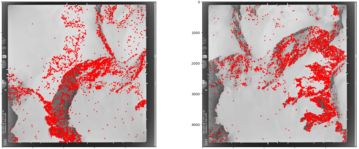
Phase 2: Extraction
The script loops through every tile and feeds it into SuperPoint. The model outputs keypoint coordinates, confidence scores, and descriptors. The local tile coordinates are then shifted back to reflect their true position on the full-resolution image.

Phase 3: Global Merge & Cleanup
Results from all tiles are concatenated into three master lists (keypoints, scores, descriptors). Because tiles overlap, the same physical feature may be detected twice. A KDTree searches for points within a 2-pixel radius of each other and removes the duplicate with the lower confidence score.

from scipy.spatial import cKDTree

# 1. Sort by score descending to prioritize high-confidence points
sort_idx = np.argsort(scores_global)[::-1]
kpts_sorted = kpts_global[sort_idx]
scores_sorted = scores_global[sort_idx]
descs_sorted = descs_global[sort_idx]

# 2. Build KDTree for efficient radius searches
tree = cKDTree(kpts_sorted)
suppression_radius = 2.0

# query_pairs finds all pairs (i, j) within the radius where i < j.
# Because we sorted by score, 'i' is always the better point.
# We can safely drop 'j' every time.
pairs = tree.query_pairs(suppression_radius)

drop_mask = np.zeros(len(kpts_sorted), dtype=bool)
for i, j in pairs:
    drop_mask[j] = True

final_kpts = kpts_sorted[~drop_mask]
final_scores = scores_sorted[~drop_mask]
final_descs = descs_sorted[~drop_mask]

If the total number of extracted points exceeds the allowed maximum, the script sorts by confidence and keeps only the top N.

Matching Keypoints

Phase 1: Global Baseline Matching
The script takes a subset of the highest-scoring keypoints from both images and runs a fast global match to establish a rough baseline for how the two images relate to one another. The larger image is designated the “base” and the smaller the “other.” If too few matches are found, the script can either stop or proceed with a more lenient threshold, depending on how you want to handle edge cases.

Phase 2: Targeted Cropping
Rather than matching everything exhaustively (O(N²) complexity), the script uses the baseline matches to calculate where each base tile lands in the second image, then draws a bounding box around that region. Only that specific area is passed to the heavy-duty matcher, which both speeds up processing and reduces false positives by narrowing the search space.

# 1. Identify which baseline matches fall within the current tile
# tile_bounds = (min_x, max_x, min_y, max_y)
mask = (
    (initial_matches['pts1'][:, 0] >= tile_bounds[0]) &
    (initial_matches['pts1'][:, 0] <  tile_bounds[1]) &
    (initial_matches['pts1'][:, 1] >= tile_bounds[2]) &
    (initial_matches['pts1'][:, 1] <  tile_bounds[3])
)

# 2. Grab the corresponding locations in Image 2
pts_in_image2 = initial_matches['pts2'][mask]

if len(pts_in_image2) == 0:
    return None  # No baseline matches to guide us

# 3. Calculate the bounding box in Image 2
min_x, max_x = pts_in_image2[:, 0].min(), pts_in_image2[:, 0].max()
min_y, max_y = pts_in_image2[:, 1].min(), pts_in_image2[:, 1].max()

# 4. Add padding so we don't miss keypoints near the edges
width_pad  = (max_x - min_x) * padding
height_pad = (max_y - min_y) * padding

x_range = (min_x - width_pad, max_x + width_pad)
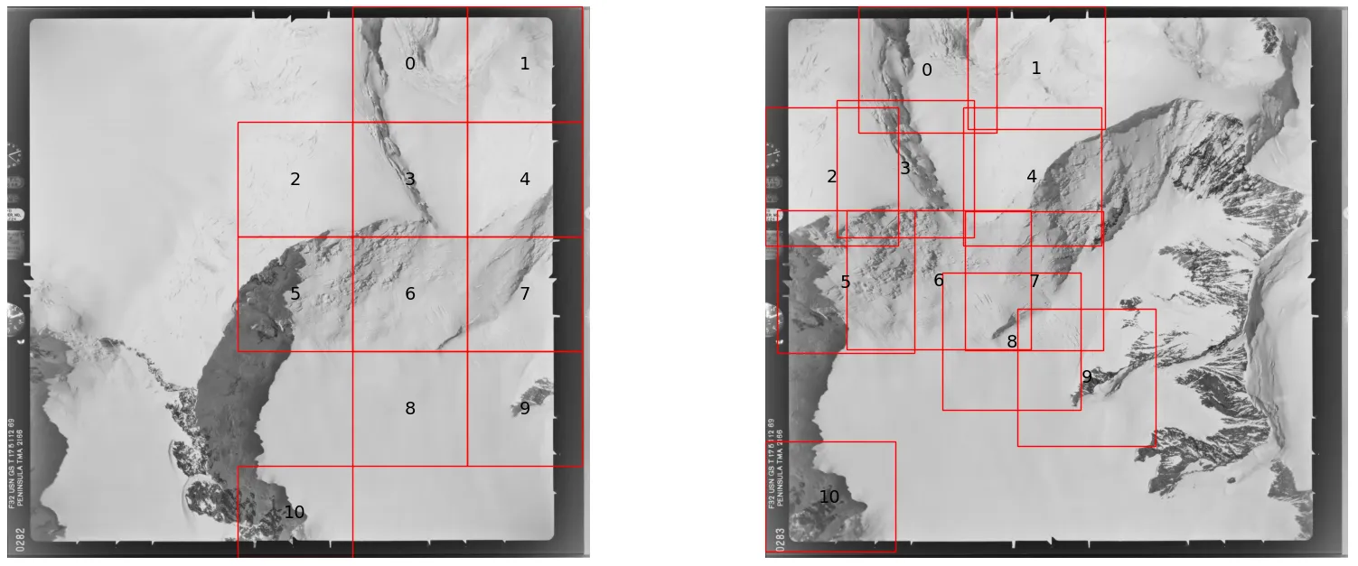
y_range = (min_y - height_pad, max_y + height_pad)

Figure 3 shows the tiles produced in this phase. The tiles in the base image are uniformly spaced, but in the second image they follow the distribution of the baseline tie points and cluster around regions of interest. The algorithm isn’t perfect—tile 8 is slightly misplaced due to an outlier in the baseline matches. One mitigation is to use only the 95th-percentile matches when computing the bounding boxes.

Phase 3: Batched Inference & Merging
The paired tile regions are grouped into batches and sent to the GPU for inference. LightGlue analyzes each targeted area to find dense, high-quality matches. If the GPU runs out of memory, the script catches the error and falls back to processing tiles one at a time. All matches from across the batches are then merged with the initial baseline matches.

Phase 4: Deduplication & Geometric Verification
A strict one-to-one mapping is enforced: if a point in Image 1 is accidentally matched to multiple points in Image 2, only the highest-confidence match survives. A spatial cleanup then removes any remaining near-duplicate matches.

# Sort by descending certainty so the best match always wins
order      = np.argsort(-certainty)
tie_points = tie_points[order]
certainty  = certainty[order]
kpts1      = tie_points[:, :2]

# Pre-compute all neighbour lists in one parallelized call
tree           = cKDTree(kpts1)
neighbor_lists = tree.query_ball_point(kpts1, r=radius, workers=-1)

kept = np.ones(len(tie_points), dtype=bool)
for i, neighbors in enumerate(neighbor_lists):
    if not kept[i]:
        continue
    for nb in neighbors:
        if nb > i:  # nb has lower certainty → suppress it
            kept[nb] = False

tie_points = tie_points[kept]
certainty  = certainty[kept]

# Simplified for brevity — see full code for complete arguments
h, inlier_mask = cv2.findHomography(...)

if h is None or inlier_mask is None:
    tie_points = np.empty((0, 4))
    certainty  = np.empty((0,))
else:
    inliers    = inlier_mask.ravel().astype(bool)
    tie_points = tie_points[inliers]
    certainty  = certainty[inliers]

Finally, a strict geometric verification using the Fundamental Matrix is run across the full merged set to remove any remaining outliers.

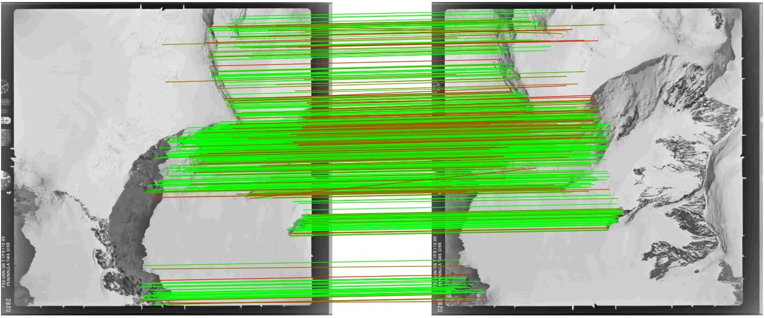
Result:

---

Approach 2: The One-Stage “Direct Tie-Point” Detector

This approach skips the independent extraction phase entirely. Instead, it pairs specific image regions up front and extracts tie points directly, using LightGlue as a fast gatekeeper and RoMa for dense, subpixel-accurate matching.

Phase 1: Initial Matchability Check
A fast LightGlue match is run at reduced resolution (around 1024px on the longest side) to check whether the images are matchable at all. If the number of inliers falls below a threshold, the script can stop early or proceed with a more lenient threshold, depending on your preference for edge cases.

One additional challenge with aerial imagery is that images can have significant relative rotation — a plane doesn’t always fly the same heading. To handle this, the pipeline first tests four candidate rotations (0°, 90°, 180°, 270°) at low resolution using LightGlue, picks the combination that yields the most geometric inliers, and applies that rotation before any tiling begins.

Phase 2: Targeted Tile Projection
The low-res matches are scaled back up to full-resolution coordinates and used to compute a global homography. Image 1 is then divided into overlapping square tiles, and for each tile, the homography is used to predict exactly where that tile appears in Image 2—avoiding the need to exhaustively check every possible tile combination.

# Simplified for brevity — see full code for complete arguments
h_full, _ = cv2.findHomography(...)

tiles_base = tile_image(base_image)

pairs = []
for box in tiles_base:
    x0_base, y0_base, x1_base, y1_base = box
    cx = (x0_base + x1_base) / 2.0
    cy = (y0_base + y1_base) / 2.0

    # Project the tile centre through H_full into the other image
    pt   = np.array([[[cx, cy]]], dtype=np.float64)
    proj = cv2.perspectiveTransform(pt, h_full)[0, 0]
    px, py = float(proj[0]), float(proj[1])

    # Skip if the projected centre falls outside the other image
    if not (0 <= px < w_other and 0 <= py < h_other):
        continue

    x0_other = int(np.clip(round(px - half), 0, max(0, w_other - tile_size)))
    y0_other = int(np.clip(round(py - half), 0, max(0, h_other - tile_size)))
    x1_other = min(x0_other + tile_size, w_other)
    y1_other = min(y0_other + tile_size, h_other)

    pairs.append((box, (x0_other, y0_other, x1_other, y1_other)))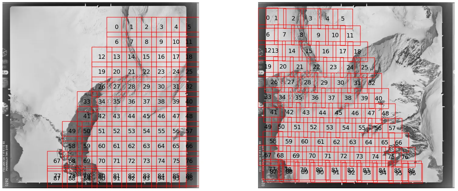

Phase 3: Dense Tile Matching
For each tile pair, SuperPoint and LightGlue run first. If they find enough seed matches, the pair is passed to RoMa for dense matching.

Phase 4: Per-Tile Cleanup
RoMa matches are filtered using a local geometric check, then spatially subsampled to prevent matches from clustering in one region. Coordinates are shifted from local tile space back to global image coordinates.

Phase 5: Global Merge & Deduplication
All tile results are concatenated into a single list. Overlapping tiles will have produced duplicate matches, which are resolved using a KDTree—keeping the higher-confidence match wherever two points fall within the deduplication radius.

Phase 6: Final Geometric Verification
A strict Fundamental Matrix check across the full merged set removes any remaining outliers.

Result:

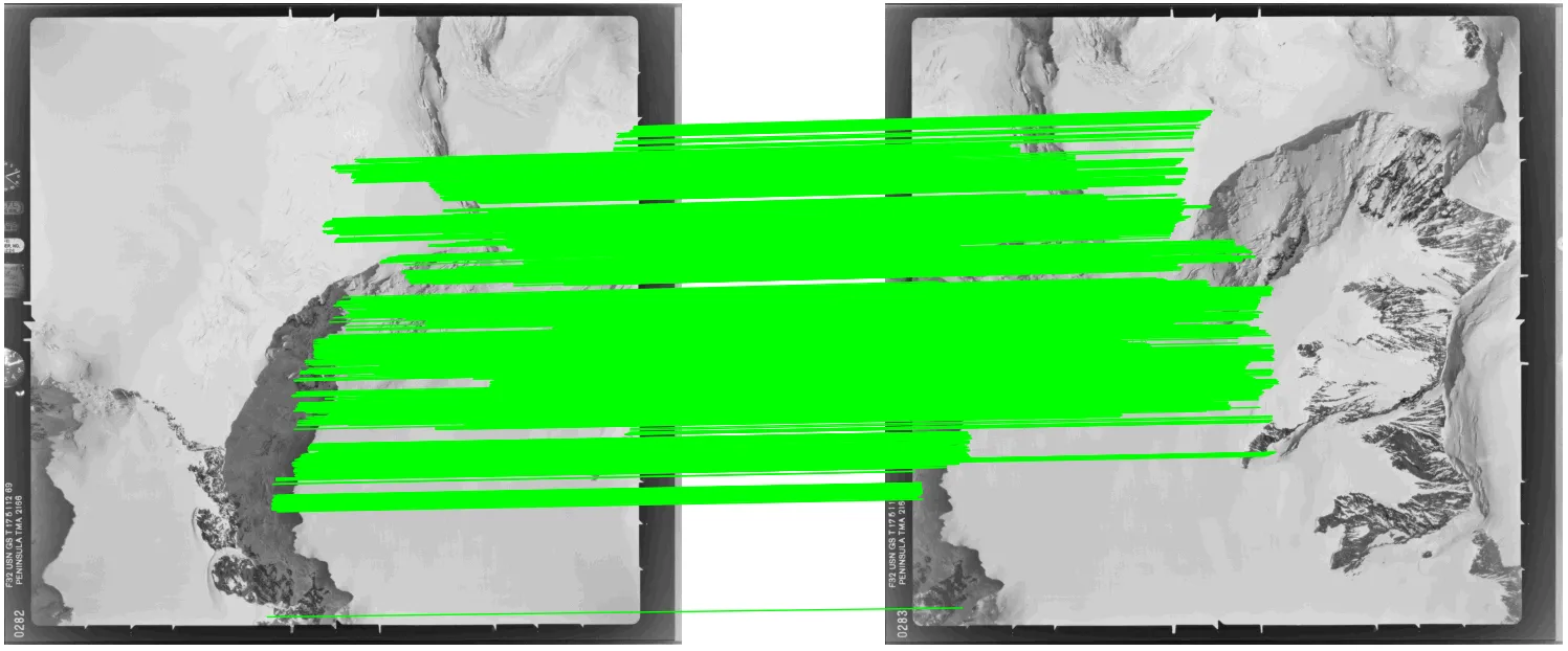
Approach 2 finds far more matches (5000 vs 776), but more isn’t always better—Approach 1 already describes the image relationship well enough for most photogrammetry workflows. It’s also worth noting that RoMa’s confidence scores carry less comparative meaning than LightGlue’s. RoMa uses importance-weighted sampling — it draws more matches from high-certainty regions — so scores naturally cluster near 1.0 and don’t discriminate between good and great matches the way LightGlue’s scores do.

---

Tips & Tricks

Overlapping tiles
Always build overlap into your tiling grid. When you slice an image into rigid squares, you risk cutting straight through important geometric features that happen to lie on a boundary. Forcing tiles to overlap (typically 10–20%) ensures every feature is fully preserved in at least one tile, which meaningfully increases match quality along the seams.

OOM handling
LightGlue and RoMa are memory-hungry, and their VRAM usage spikes unpredictably depending on the visual complexity of each tile pair. To prevent a single dense tile from crashing a multi-hour run, wrap your inference calls in a targeted try-except block.

try:
    run_matching_on_gpu()

except torch.cuda.OutOfMemoryError as e:
    print(f"OOM caught: {e}")
    torch.cuda.empty_cache()

    # Fall back to CPU, lower resolution, or reduced batch size
    print("Falling back to reduced resolution...")
    return None

except Exception as e:
    raise e  # Re-raise anything that isn't an OOM

Subpixel accuracy for SuperPoint/LightGlue
SuperPoint and LightGlue are inherently limited to pixel-level precision, but subpixel refinement can be applied as a post-processing step. One option I’ve found effective is keypt2subpx, which plugs in after the matching step with minimal overhead. It improves results noticeably but is not a full substitute for a natively subpixel method like RoMa.

---

Conclusion

Matching high-resolution aerial imagery is a balancing act between computational efficiency and geometric precision. Modern matchers like LightGlue and RoMa have transformed what’s possible on difficult textures and lighting conditions, but they need a thoughtful tiling strategy around them to operate at scale without running out of memory or losing accuracy.

The two approaches here offer different paths to that goal. Approach 1 is efficient and reusable, well-suited to standard batch workflows. Approach 2 is the heavy-duty alternative for cases where subpixel accuracy and high match density are non-negotiable.

Room for improvement
Both pipelines are still evolving. Areas I’m actively looking to refine:

• Rotation invariance: The current tile projection works best for images with limited relative rotation. When images are significantly rotated, the projected bounding boxes inflate well beyond the true overlap region, wasting computation and reducing matching precision.
• Planar scene assumption: The homography-based tile projection assumes a flat scene. For imagery with significant elevation variation—mountainous terrain, for instance—this breaks down. A local affine model per tile or depth-guided warping would be more robust.

In practice, both pipelines have held up on some of the most hostile imagery I’ve encountered: near-featureless Antarctic ice fields captured on decades-old film, with all the grain, fading, and geometric distortion that comes with it. If they work there, they should serve you well on more forgiving material.

If you’re exploring this space, I also highly recommend DEEP-IMAGE-MATCHING, which incorporates several of the strategies discussed here and is actively maintained.